Estimating volcanic SO2 flux - Volcano Space Observatory

To estimate SO2 flux released by volcanoes, we will use the “disk method”, introduced in Grandin et al. (2024).

The algorithm is available in open-source from ICARE’s GitLab https://git.icare.univ-lille.fr/icare-public/so2-flux-calculator

The code can be installed using the following command:

pip install 'so2-flux-calculator[test,interactive,ecmwfapi]' --index-url https://git.icare.univ-lille.fr/api/v4/projects/661/packages/pypi/simple

Below is a quick introduction of the principle of the method

Idealized model of a SO2 plume¶

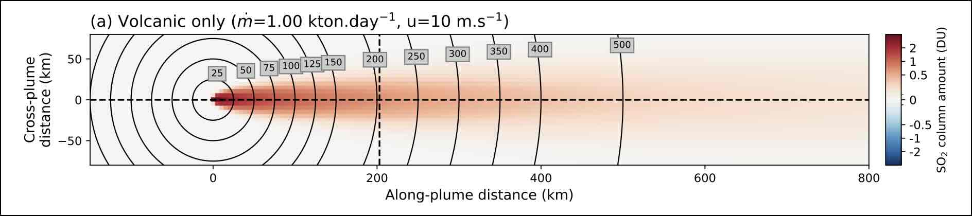
The method starts with a simplified model describing the distribution of column amount released by a point source:

D(x,y) = \int C(x,y,z)\; \mathrm{d}z = \dfrac{\dot{m}/u}{\sqrt{4 \pi D_y (x/u)}}.\exp{\left\{ \dfrac{-uy^2}{4 D_y x} \right\}}.\exp{\left\{ \dfrac{-kx}{u}\right\}}

(1)

where:

$C$ : SO2 concentration (local)
$D$ : SO2 column amount (integrated in the vertical direction)
$x, y$ : cartesian coordinates
$u$ : wind speed
$\dot{m}$ : SO2 mass flux from the source
$k$ : (inverse) decay rate due to SO2 degradation
$D_x, D_y$ : diffusion coefficients

This expression is a simplified solution of the advection-diffusion equation, commonly named a “gaussian plume”.

Mass versus distance¶

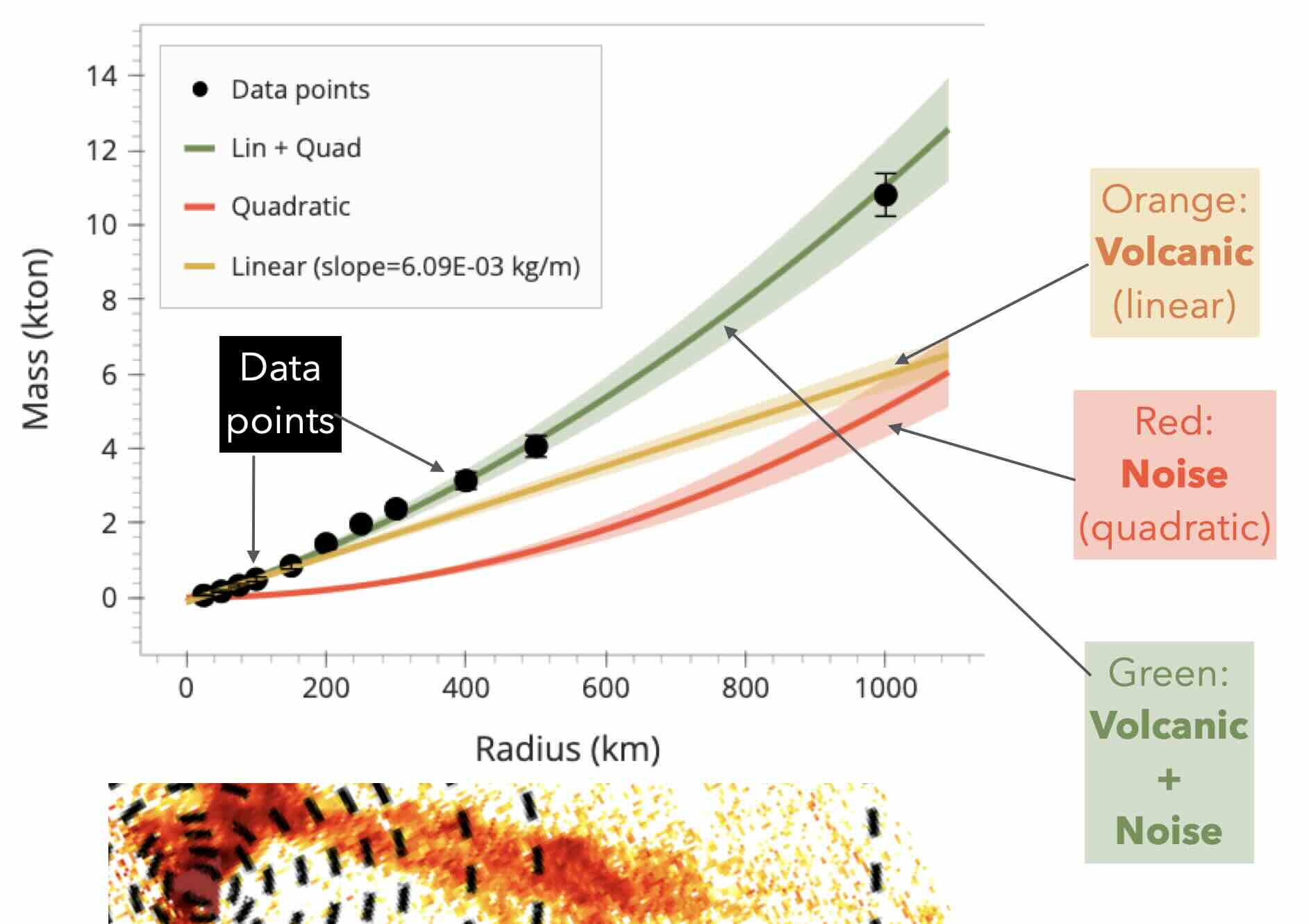
Integrating Equation (1) as a function of distance $r$ from the source gives the following integrated-mass-to-distance expression:

M_{volc}(r)= \iint_{R=0}^{R=r} D(R)\mathrm{d}S \approx \int_{x=0}^{x=r} \int_{y=-\infty}^{y=+\infty}D(x,y) \:\mathrm{d}x\mathrm{d}y = \dfrac{\dot{m}}{k} \left( 1 - \exp{\left\{ \dfrac{- k r}{u}\right\}} \right)

(2)

A first-order expansion of Equation (2) yields a simplified result:

M_{volc}(r)\approx\dfrac{\dot{m}}{u}r

(3)

This expression states that integrated mass $M$ is proportional to distance $r$ from the source. The proportionality factor, $\dot{m}/u$ is a quantity named the “proto-flux”, which is defined as the ratio of the SO2 mass flux ( $\dot{m}$ ) and wind velocity ( $u$ ).

The importance of noise¶

This idealized model is perturbed by two additional factors that cannot be avoided when working with real data:

data is noisy
users typically mask out pixels with “low” SO2 concentrations, which are considered as meaningless (a process called “truncation”)

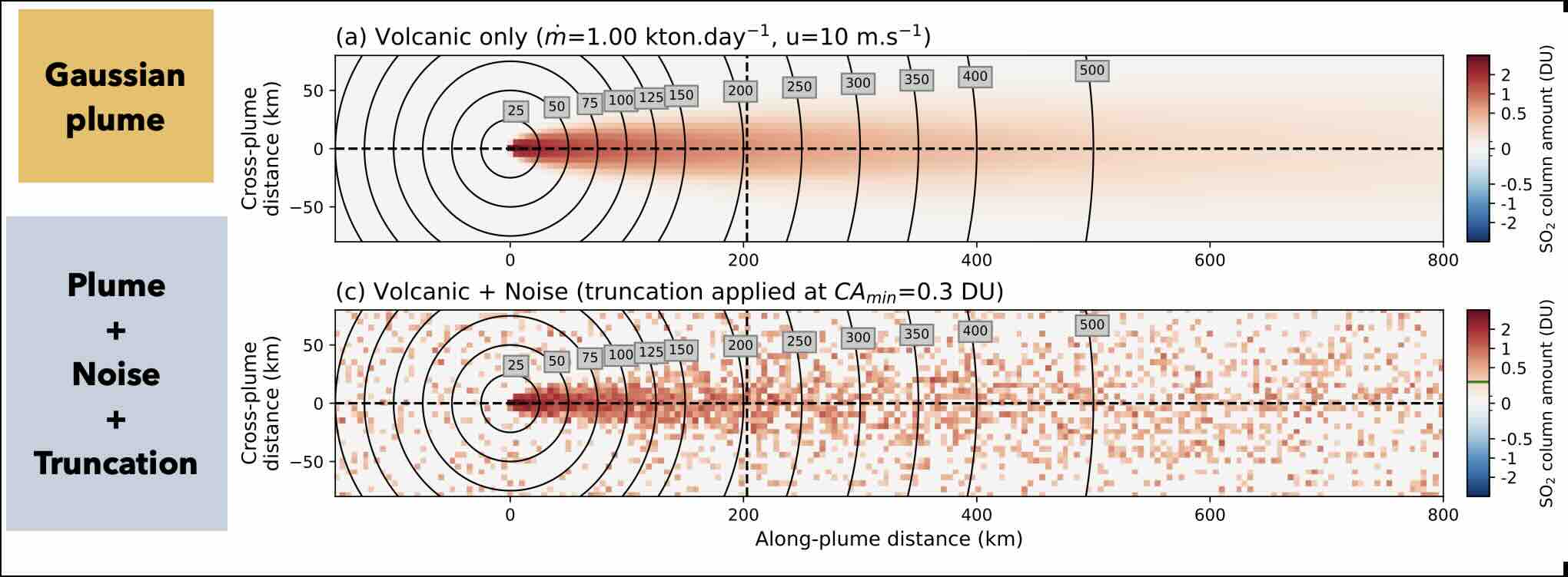
This situation can be modeled using a truncated gaussian probability function, which introduces a quadratic term in Equation (3):

\begin{align*} M(r) &=& M_{volc}(r)& + &M_{noise}(r)\\ &=& \dfrac{\dot{m}}{u}r &+& b.r^2 \end{align*}

(4)

Therefore, the estimation procedure consists in performing a regression, where :

the linear factor is the volcanic “proto-flux”
the quadratic term is the “noise”.

Recap: main steps of the method¶

estimate $\dot{m}/u$ from TROPOMI data, along with the noise term, by regression
multiply the “proto-flux” by wind speed $u$
the final result if the SO2 mass flux $\dot{m}$

Key simplifications¶

fixed source
constant wind
constant mass flux
along-plume diffusion is neglected compared to plume transport (Low Péclet number)
truncated gaussian noise model
separability of the linear and quadratic terms of the regression

References¶

Grandin, R., Boichu, M., Mathurin, T., & Pascal, N. (2024). Automatic Estimation of Daily Volcanic Sulfur Dioxide Gas Flux From TROPOMI Satellite Observations: Application to Etna and Piton de la Fournaise. Journal of Geophysical Research: Solid Earth, 129(6). 10.1029/2024jb029309

Volcano Space Observatory

TROPOMI data

Volcano Space Observatory

Compute SO2 mass