Last update 👈
David Palecek, August 12, 2025
Many campaigns have been analysed with MGnify pipeline. EMO-BON data use metaGOflow pipeline, which is a reads subworkflow of the MGnify. Therefore the summury tables available at MGnify are directly comparable with the EMO-BON metaGOflow outputs.
Here we (a) select several campaigns related to the European region at MGnify, (b) query taxonomic sumaries for the whole campaign based on the study ID and (c) provide an overview visualization.
Overall, this is a starting point for taxonomic universal comparison engine for Mgnify outputs.
Note
Even though the function to query the data via the API is provided below, we use pre-downloaded files here.
Setup and data loading
import os
import warnings
warnings.filterwarnings('ignore')

from functools import partial

import numpy as np
import pandas as pd
import matplotlib.pyplot as plt

from dotenv import load_dotenv
load_dotenv()

# All low level functions are imported from the momics package
from momics.utils import load_and_clean

from momics.taxonomy import (
    fill_taxonomy_placeholders,
    pivot_taxonomic_data,
    prevalence_cutoff,
    clean_tax_row,
)

# allows plotting of venn diagrams of 4 sets
from venny4py.venny4py import *
Below is the method used to query and save. Run it in the loop if you have a list of studies to download
from jsonapi_client import Session as APISession
from urllib.request import urlretrieve

def retrieve_summary(studyId: str, matching_string: str = 'Taxonomic assignments SSU') -> None:
    """
    Retrieve summary data for a given analysis ID and save it to a file. Matching strings
    are substrings of for instance:
    - Phylum level taxonomies SSU
    - Taxonomic assignments SSU
    - Phylum level taxonomies LSU
    - Taxonomic assignments LSU
    - Phylum level taxonomies ITSoneDB
    - Taxonomic assignments ITSoneDB
    - Phylum level taxonomies UNITE
    - Taxonomic assignments UNITE

    Example usage:
    retrieve_summary('MGYS00006680', matching_string='Taxonomic assignments SSU')

    Args:
        studyId (str): The ID of the analysis to retrieve. studyId is the MGnify study ID, used
            also to save the output .tsv file.
        matching_string (str): The string to match in the download description label.

    Returns:
        None
    """
    with APISession("https://www.ebi.ac.uk/metagenomics/api/v1") as session:
        for download in session.iterate(f"studies/{studyId}/downloads"):
            if download.description.label == matching_string:
                print(f"Downloading {download.alias}...")
                urlretrieve(download.links.self.url, f'{studyId}.tsv')
# example of execution
retrieve_summary('MGYS00006680', matching_string='Taxonomic assignments SSU')SSU table is used for this demonstration, but the methods shows are agnostic to taxonomic table origin. Metadata are not treated in this example, because their harmonization requires tedious manual work.
def get_valid_samples():
    url = "https://raw.githubusercontent.com/emo-bon/momics-demos/refs/heads/main/data/shipment_b1b2_181.csv"
    df_valid = pd.read_csv(
        url, header=0, index_col=0,
    )
    return df_valid

valid_samples = get_valid_samples()

# load data
full_metadata, mgf_parquet_dfs = load_and_clean(valid_samples=valid_samples)
ssu = mgf_parquet_dfs['ssu'].copy()
del mgf_parquet_dfs

ssu.head()Define a taxonomy rank strings as a global variable
TAXONOMY_RANKS = ['superkingdom', 'kingdom', 'phylum', 'class', 'order', 'family', 'genus', 'species']Pivot EMO-BON data
EMO-BON taxonomy tables
# fill missing higher taxa (usually happens for tentative taxa)
ssu_filt = fill_taxonomy_placeholders(ssu, TAXONOMY_RANKS)

## pivot the abundance table
ssu_filt = pivot_taxonomic_data(ssu_filt)

# unify taxonomic information to the MGnify
ssu_filt = ssu_filt.reset_index()
ssu_filt['taxonomic_concat'] = ssu_filt['taxonomic_concat'].apply(clean_tax_row)

# unify column and index names
ssu_filt = ssu_filt.set_index('ncbi_tax_id')
ssu_filt = ssu_filt.rename(columns={
    'taxonomic_concat': '#SampleID',
})

ssu_filt.head()Process MGnify datasets
The list of selected datasets is far from exhausted but includes:
| Study ID | Description |
|---|---|
| MGYS00006608 | 16S rRNA amplicon sequencing from the Ocean Sampling Day (OSD), June 2018 |
| MGYS00006607 | 16S rRNA amplicon sequencing from the Ocean Sampling Day (OSD), June 2019 |
| MGYS00000492 | Amplicon sequencing of Tara Oceans DNA samples corresponding to size fractions for prokaryotes or protist |
| MGYS00006680 | SOLA sampling point Raw sequence reads |
| MGYS00006682 | Vertical stratification of environmental DNA in the open ocean captures ecological patterns and behavior of deep-sea fishes |
| MGYS00006678 | Dataset on spatiotemporal variation of microbial plankton communities in the Baltic Sea |
| MGYS00006675 | 16S rRNA gene amplicon time-series in Blanes Bay Microbial Observatory (BBMO) |
| MGYS00003725 | Arctic microbiome along Svalbard Cross Shelf transects |
| MGYS00006686 | Environmental DNA and zooplankton samples taken at Helgoland Roads in June 2019 |
| MGYS00006714 | Regional and vertical patterns in microbial communities across Fram Strait (2015-2019) |
ds_list = {
    'OSD-2018': 'mgnify_data/ERP124424_taxonomy_abundances_SSU_v5.0.tsv',
    'OSD-2019': 'mgnify_data/ERP124431_taxonomy_abundances_SSU_v5.0.tsv',
    'Tara': 'mgnify_data/ERP003634_taxonomy_abundances_SSU_v5.0.tsv',
    'Sola': 'mgnify_data/SRP237882_taxonomy_abundances_SSU_v5.0.tsv',
    'Biscay': 'mgnify_data/SRP334933_taxonomy_abundances_SSU_v5.0.tsv',
    'Baltic': 'mgnify_data/ERP140185_taxonomy_abundances_SSU_v5.0.tsv',
    'BBMO': 'mgnify_data/ERP122219_taxonomy_abundances_SSU_v5.0.tsv',
    'Svalbard': 'mgnify_data/ERP106348_taxonomy_abundances_SSU_v5.0.tsv',
    'Helgoland': 'mgnify_data/ERP144826_taxonomy_abundances_SSU_v5.0.tsv',
    'Fram': 'mgnify_data/ERP151329_taxonomy_abundances_SSU_v5.0.tsv',
}

# loading tsv tables
ds = {}
for key, value in ds_list.items():
    url = f"https://raw.githubusercontent.com/fair-ease/book-marine-omics-observation/refs/heads/main/book/assets/data/{value}"
    df = pd.read_csv(url, sep="\t", header=0)
    # df = pd.read_csv(os.path.join(data_folder, value), sep='\t')
    df['#SampleID'] = df['#SampleID'].apply(clean_tax_row)
    print(key, f"Dataframe shape (rows, columns): {df.shape}")
    ds[key] = df
OSD-2018 Dataframe shape (rows, columns): (1981, 63)
OSD-2019 Dataframe shape (rows, columns): (1708, 49)
Tara Dataframe shape (rows, columns): (497, 8)
Sola Dataframe shape (rows, columns): (3484, 284)
Biscay Dataframe shape (rows, columns): (118, 53)
Baltic Dataframe shape (rows, columns): (4316, 666)
BBMO Dataframe shape (rows, columns): (2503, 250)
Svalbard Dataframe shape (rows, columns): (1505, 82)
Helgoland Dataframe shape (rows, columns): (2241, 166)
Fram Dataframe shape (rows, columns): (1428, 206)
Note
loading the data from GitHub is a consequence of inability of the book executed on binder to reference “local files” using relative references.
Normalize the abundance tables, either with total sum scaling (tss) with possible square root (tss_sqrt).
def normalize_taxonomy(df, method: str = 'tss'):
    """
    Normalize the taxonomy dataframe by removing high taxa and applying prevalence cutoff.
    """
    if method == 'tss':
        df.iloc[:, 1:] = df.iloc[:, 1:].apply(lambda x: x / x.sum())
    elif method == 'tss_sqrt':
        df.iloc[:, 1:] = df.iloc[:, 1:].apply(lambda x: (x / x.sum()) ** 0.5)
    else:
        raise ValueError("Normalization method not recognized. Use 'tss' or 'tss_sqrt'.")
    return df

# add emo-bon to the dataset dictionary
ds['EMO-BON'] = ssu_filt.copy()

ds_normalized = {}
for key, value in ds.items():
    df = value.copy()
    df = prevalence_cutoff(df, percent=0.1, skip_columns=1)
    df = normalize_taxonomy(df, method='tss')
    ds_normalized[key] = df
Most abundant taxa in the dataset
top_species = []
for i, (label, df_orig) in enumerate(ds_normalized.items()):
    df = df_orig.copy()
    # first sum off the samples ie columns
    df['sum'] = df.iloc[:, 1:].sum(axis=1) / (len(df.columns)-1) *100
    # then sort by sum
    df = df.sort_values(by='sum', ascending=False)

    # keep only the top X species
    df = df.head(5)

    for j, val in enumerate(df['#SampleID']):
        top_species.append(val.split(";")[-1])
top_species = list(set(top_species))

print("Top species occuring over all the datasets")
print(top_species)
Top species occuring over all the datasets
['sk__Bacteria', 'f__Oikopleuridae', 'f__Rhodobacteraceae', 'f__Flavobacteriaceae', 's__Acartia_clausii', 'c__Deltaproteobacteria', 'c__Alphaproteobacteria', 'sk__Eukaryota', 'p__Cyanobacteria', 'c__Dehalococcoidia', 'o__Pelagibacterales', 'p__Thaumarchaeota', 'o__Calanoida', 'c__Spirotrichea', 'c__Gammaproteobacteria', 'p__Arthropoda']
Associate a colorscheme with the list of species
# Choose a colormap and normalize the color range
cmap = plt.get_cmap('jet')
norm = plt.Normalize(0, len(top_species) - 1)

# Map each item to a color
color_dict = {name: cmap(norm(i)) for i, name in enumerate(top_species)}

# Example: print or use a color
print(color_dict)
{'sk__Bacteria': (np.float64(0.0), np.float64(0.0), np.float64(0.5), np.float64(1.0)), 'f__Oikopleuridae': (np.float64(0.0), np.float64(0.0), np.float64(0.803030303030303), np.float64(1.0)), 'f__Rhodobacteraceae': (np.float64(0.0), np.float64(0.03333333333333333), np.float64(1.0), np.float64(1.0)), 'f__Flavobacteriaceae': (np.float64(0.0), np.float64(0.3), np.float64(1.0), np.float64(1.0)), 's__Acartia_clausii': (np.float64(0.0), np.float64(0.5666666666666667), np.float64(1.0), np.float64(1.0)), 'c__Deltaproteobacteria': (np.float64(0.0), np.float64(0.8333333333333334), np.float64(1.0), np.float64(1.0)), 'c__Alphaproteobacteria': (np.float64(0.16129032258064513), np.float64(1.0), np.float64(0.8064516129032259), np.float64(1.0)), 'sk__Eukaryota': (np.float64(0.3763440860215053), np.float64(1.0), np.float64(0.5913978494623656), np.float64(1.0)), 'p__Cyanobacteria': (np.float64(0.5913978494623655), np.float64(1.0), np.float64(0.3763440860215054), np.float64(1.0)), 'c__Dehalococcoidia': (np.float64(0.8064516129032256), np.float64(1.0), np.float64(0.16129032258064513), np.float64(1.0)), 'o__Pelagibacterales': (np.float64(1.0), np.float64(0.9012345679012348), np.float64(0.0), np.float64(1.0)), 'p__Thaumarchaeota': (np.float64(1.0), np.float64(0.6543209876543212), np.float64(0.0), np.float64(1.0)), 'o__Calanoida': (np.float64(1.0), np.float64(0.40740740740740755), np.float64(0.0), np.float64(1.0)), 'c__Spirotrichea': (np.float64(1.0), np.float64(0.16049382716049398), np.float64(0.0), np.float64(1.0)), 'c__Gammaproteobacteria': (np.float64(0.8030303030303032), np.float64(0.0), np.float64(0.0), np.float64(1.0)), 'p__Arthropoda': (np.float64(0.5), np.float64(0.0), np.float64(0.0), np.float64(1.0))}
Visualize the most abundant taxa in each of the datasets
fig, ax = plt.subplots()
x_positions = np.arange(len(ds_normalized))  # one bar per DataFrame
bar_width = 0.5

xlabels = []
for i, (label, df_orig) in enumerate(ds_normalized.items()):
    bottom = 0
    df = df_orig.copy()
    # first sum off the samples ie columns
    df['sum'] = df.iloc[:, 1:].sum(axis=1) / (len(df.columns)-1) *100
    # print(df['sum'].sum(), len(df.columns)-2)
    # then sort by sum
    df = df.sort_values(by='sum', ascending=False)

    # keep only the top X species
    df = df.head(5)

    for j, val in enumerate(df['sum']):
        ax.bar(x_positions[i], val, bottom=bottom, width=bar_width,
               color=color_dict[df['#SampleID'].iloc[j].split(";")[-1]],
        )
        bottom += val
    xlabels.append(label)

# manual legend
handles = [plt.Rectangle((0,0),1,1, color=color_dict[name]) for name in top_species]
ax.legend(handles, top_species, loc="center left", bbox_to_anchor=(1, 0.5))
ax.set_xticks(x_positions)
ax.set_xticklabels(xlabels, rotation=45, ha='right')

ax.set_ylabel('Relative abundance in all samples pooled [%]')
ax.set_xlabel('Dataset')
ax.set_title('Most abundant taxa in each dataset')
plt.show()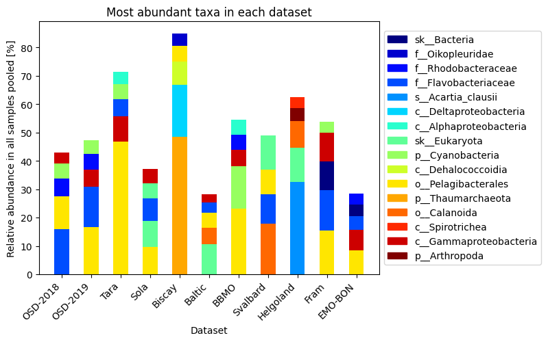
Alpha diversity
Alpha diversity measures diversity within a single sample or community, capturing both richness (How many different species (or taxa) are present) and evenness (How evenly distributed the species are)
Higher Shannon Index = more diverse community Lower Shannon Index = fewer or more unevenly distributed taxa
from momics.diversity import calculate_shannon_index

for k, v in ds.items():
    df = v.copy().T
    shannon_vals = calculate_shannon_index(df)
    plt.plot(shannon_vals, 'o', alpha=0.5, label=f'{k}-av {shannon_vals.mean():.2f}')
plt.legend(loc="center left", bbox_to_anchor=(1, 0.5))
plt.xticks([])
plt.xlabel('Sample')
plt.ylabel('Shannon index')
plt.title('Alpha diversity (Shannon index)')
plt.show()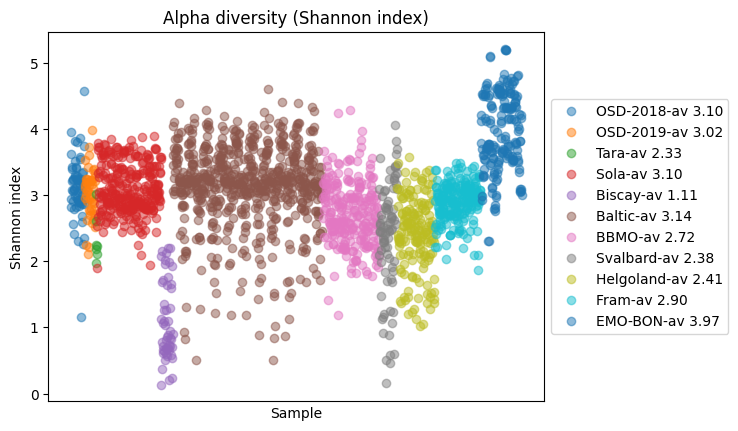
Beta diversity
Beta diversity measures differences in species composition between samples, i.e., how different are communities from each other. Alpha diversity refers to diversity of each sample, beta diversity describes how samples are different from each other.
For the pair-wise dissimilarities, we will use Bray-Curtis distance
from skbio.diversity import beta_diversity
import seaborn as sns
from skbio.stats.ordination import pcoa

pcoa_res, explained_var = {}, {}

fig, ax = plt.subplots(4, 3, figsize=(18, 10))
# starts from the normalized DS dictionary
for i, (k, v) in enumerate(ds.items()):
    df = v.set_index('#SampleID').copy().T
    beta = beta_diversity('braycurtis', df)
    #order beta
    df_beta = beta.to_data_frame()

    # this is for later use in PCoA
    pcoa_result = pcoa(df_beta, method="eigh")
    pcoa_res[k] = pcoa_result
    explained_var[k] = (
        pcoa_result.proportion_explained[0],
        pcoa_result.proportion_explained[1],
    )

    sums = df_beta.sum(axis=1)

    # Sort index by sum
    sorted_idx = sums.sort_values(ascending=False).index

    # Reorder both rows and columns
    corr_sorted = df_beta.loc[sorted_idx, sorted_idx]
    curr_ax = ax.flatten()[i]
    sns.heatmap(corr_sorted, cmap="YlGnBu", ax=curr_ax)
    curr_ax.legend(loc="center left", bbox_to_anchor=(1, 0.5))
    curr_ax.set_xticks([])
    curr_ax.set_ylabel('Sample')
    curr_ax.set_title(f'Beta div., {k}')
plt.show()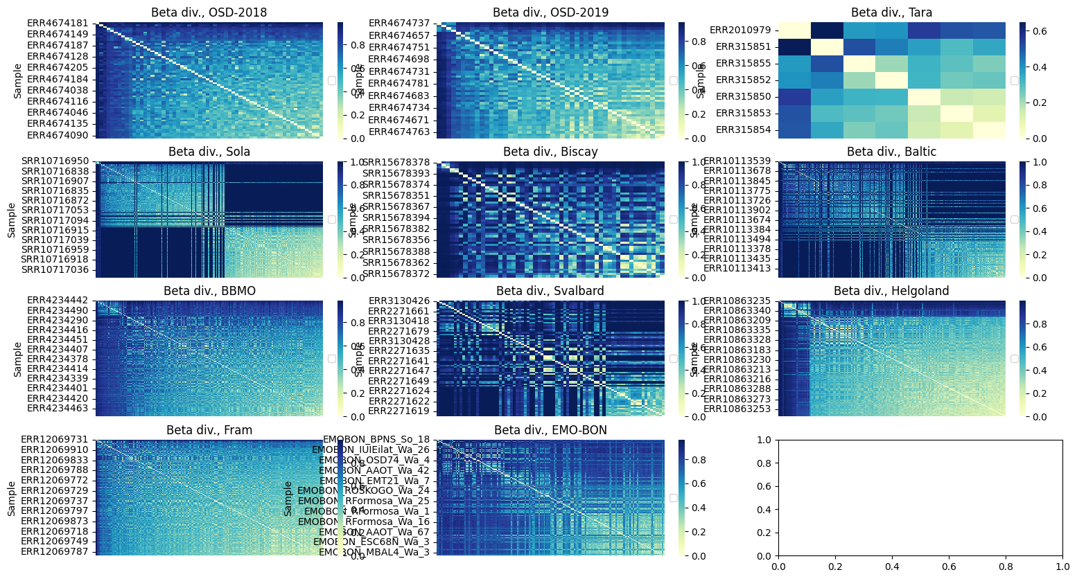
PCoA
In the previous section we have already precalcuted PCoA for samples from each campign (pcoa_result), we can therefore plot the first two components with their respective expained variances.
fig, ax = plt.subplots(3, 4, figsize=(25, 16))

for i, (k, v) in enumerate(pcoa_res.items()):
    curr_ax = ax.flatten()[i]

    sns.scatterplot(
        data=v.samples,
        x="PC1",
        y="PC2",
        ax=curr_ax,
    )
    curr_ax.set_xlabel(f"PC1 ({explained_var[k][0]*100:.2f})")
    curr_ax.set_ylabel(f"PC2 ({explained_var[k][1]*100:.2f})")
    curr_ax.set_title(f"PCoA, Bray-Curtis - {k}")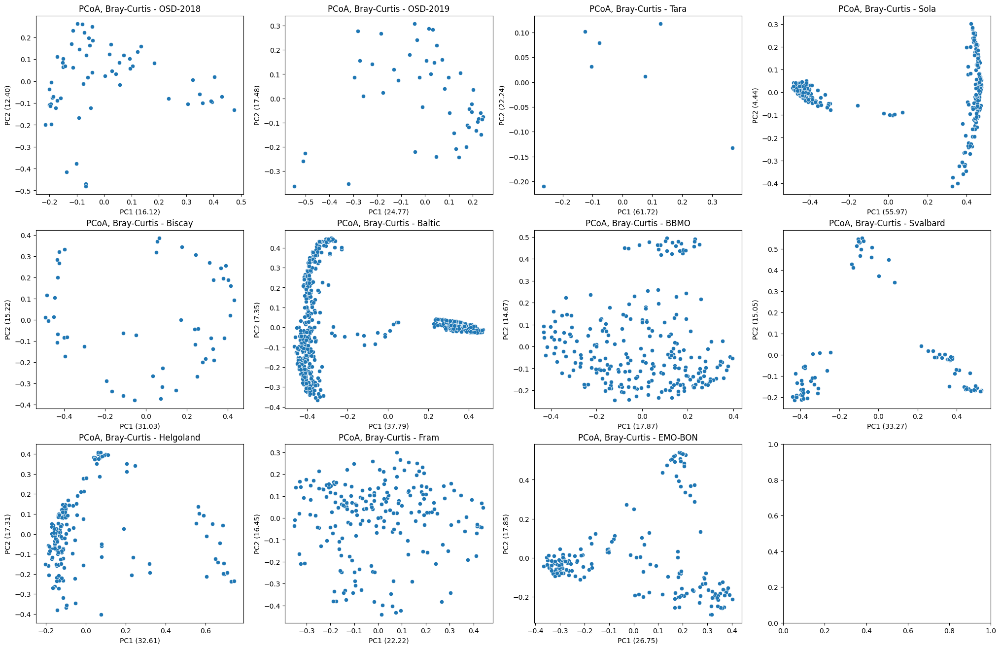
MDS and NMDS
MDS stands for Metric Multidimensional Scaling. Below, we use the scipy impolementation of the distance matrix and MDS.
from sklearn.manifold import MDS
from scipy.spatial.distance import pdist, squareform

fig, ax = plt.subplots(3, 4, figsize=(25, 16))

for i, (k, v) in enumerate(ds.items()):
    curr_ax = ax.flatten()[i]
    df = v.set_index('#SampleID').copy().T

    # Step 1: Calculate Bray-Curtis distance matrix
    # Note: pdist expects a 2D array, so we use df.values
    dist_matrix = pdist(df.values, metric='braycurtis')
    dist_square = squareform(dist_matrix)

    # Step 3: Run MDS
    mds = MDS(n_components=2, dissimilarity='precomputed', random_state=42)
    coords = mds.fit_transform(dist_square)

    # Step 4: Plot
    curr_ax.scatter(coords[:, 0], coords[:, 1], s=50)

    # Optional: label samples
    # for i, sample_id in enumerate(df.index):
    #     curr_ax.text(coords[i, 0], coords[i, 1], sample_id, fontsize=8)

    curr_ax.set_title("MDS of Bray-Curtis - " + k)
    curr_ax.set_xlabel("MDS1")
    curr_ax.set_ylabel("MDS2")
    # curr_ax.grid(True)
plt.tight_layout()
plt.show()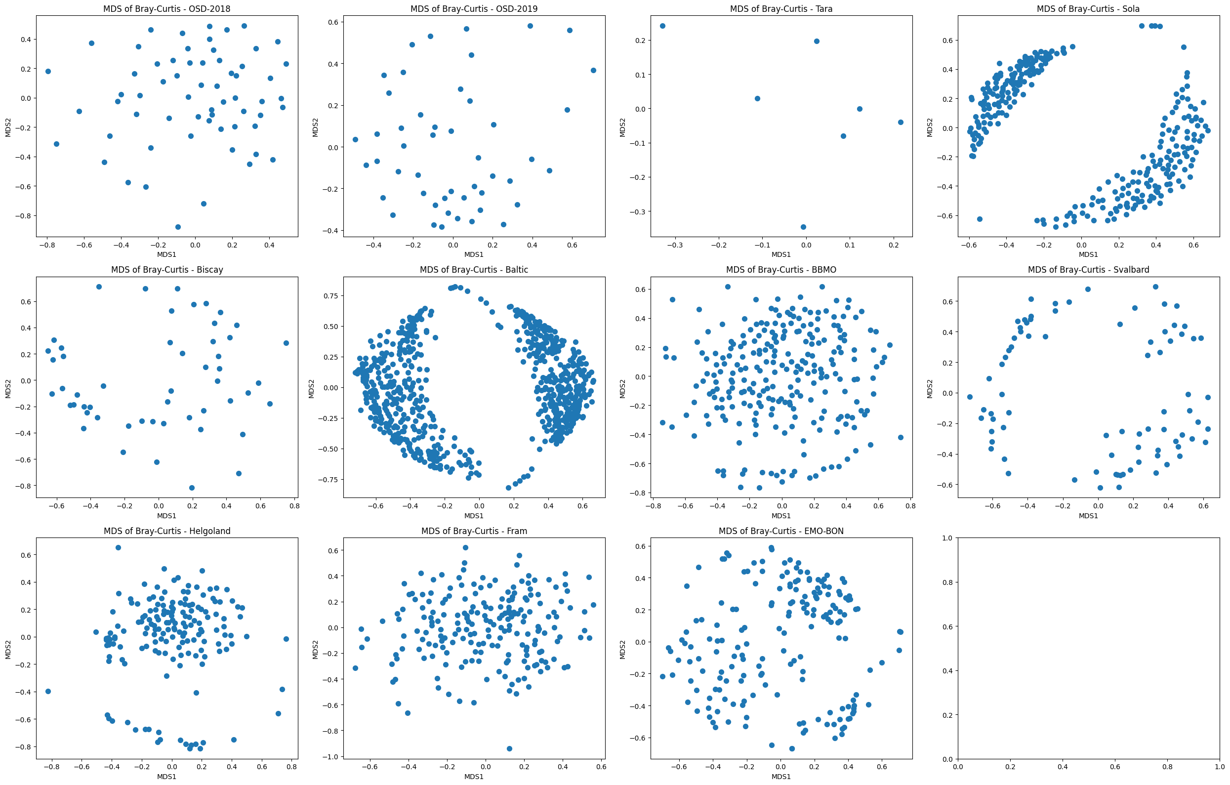
Venn diagram of taxonomic IDs overlap
#dict of sets
sets = {
    'EMO-BON': set(ds_normalized['EMO-BON']['#SampleID'].values),
    'OSD 2018': set(ds_normalized['OSD-2018']['#SampleID'].values),
    'OSD 2019': set(ds_normalized['OSD-2019']['#SampleID'].values),
    'SOLA': set(ds_normalized['Sola']['#SampleID'].values)
}

fig = venny4py(sets=sets)#, out = 'venn4.png')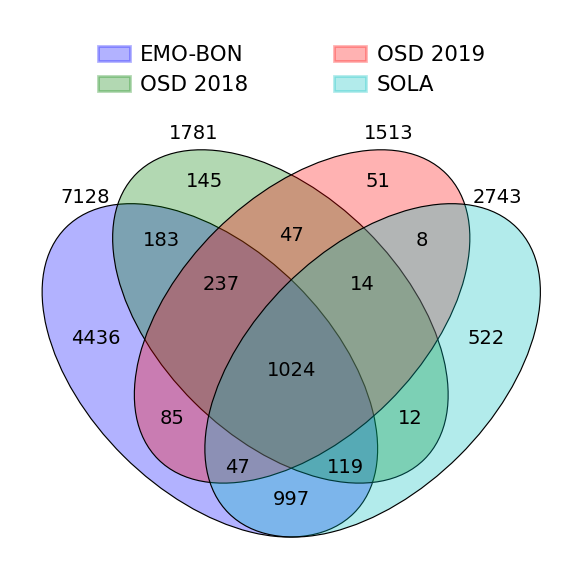
Cummulative taxa discovery along the sampling campaigns
If we consider samplings over time, how do we accumulate identified taxa? Hypothesis is, that if the dependence of discovery is not flattening out, the campaign is heavily undersampling the reality of changing microbiome at the sampling sites over time. To visualize this, below the cummulative taxa is calculated along the collection dates in the case of EMO-BON data, or simply in column order of the other campaigns.
# for other datasets I do not order by date
res_dict = {}
for key, ds in ds_normalized.items():
    cumm_taxa = set()
    res_dict[key] = [0]
    for idx in ds.columns[1:].to_list():
        data = ds[idx]  # single sampling
        positive_idx = data[data > 0].index.to_list()  # filter the once with abundance
        cumm_taxa.update(positive_idx)  # add to the set
        res_dict[key].append(len(cumm_taxa))  # append count which equals to updated set

cumm_taxa = set()
taxa_count = [0]
for idx, row in full_metadata['collection date'].sort_values().items():

    data = ds_normalized['EMO-BON'][idx]  # single sampling
    positive_idx = data[data > 0].index.to_list()  # filter the once with abundance
    cumm_taxa.update(positive_idx)  # add to the set
    taxa_count.append(len(cumm_taxa))  # append count which equals to updated set

res_dict['EMO-BON'] = taxa_count
Now it is possible to plot the cummulative taxa-count
for key, taxa_count in res_dict.items():
    plt.plot(
        taxa_count,
        label=key
    )
plt.xlabel('Collection date index')
plt.ylabel('Cumulative number of taxa')
plt.legend()
plt.show()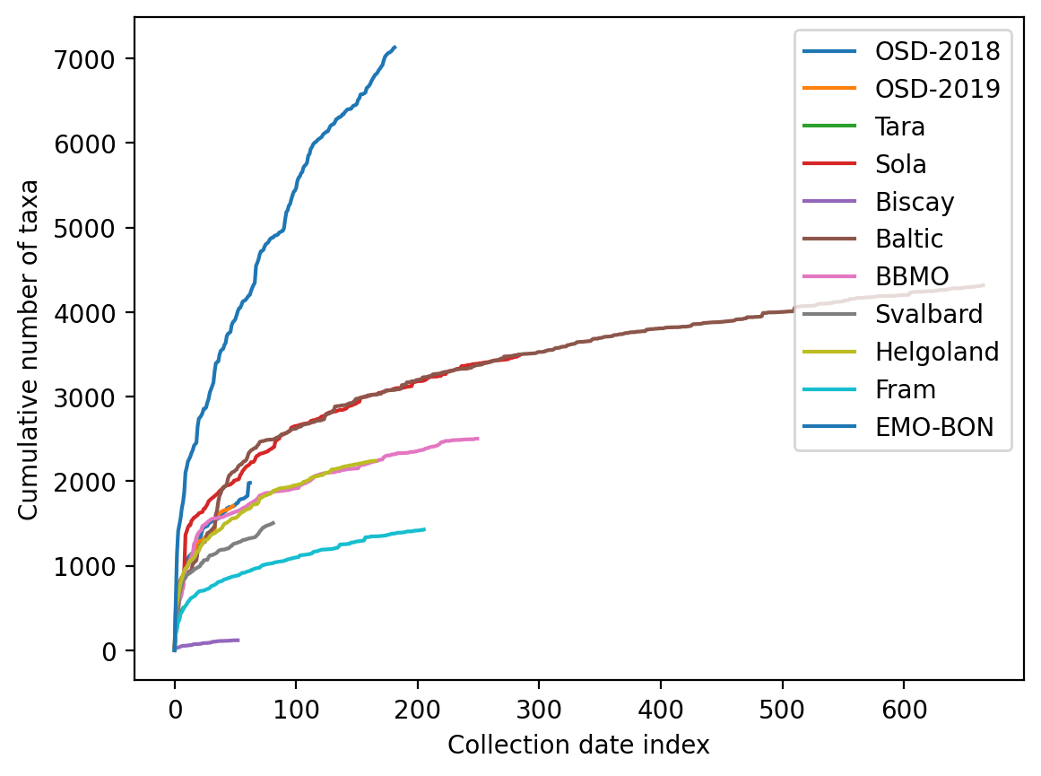
The EMO-BON campaign shows high added value in terms of new taxa being found for repeated sampling events along the time. The discovery rate is in the linear regime of the last 100 samplings.
last_x = 100
print(f'Steady rate of taxonomic discovery: {(taxa_count[-1] - taxa_count[-last_x-1]) / last_x} taxa per collection date')
Steady rate of taxonomic discovery: 22.49 taxa per collection date
It is unclear why that is, but it might be linked to sampling depth of the sequencing, which can be further confirmed.
Conclusions
EMO-BON sampling shows superior taxonomic diversity and large proportion of uniquely identified taxa in comparison to the other campaings. Sequencing depth can explain higher alpha diversity, which needs to be confirmed manually with other campaing sequencing approaches. Uniquely identified taxa underline the importance and value of long-term diversity sampling campaigns. Strong correlation between taxa identified and number of samplings suggests that we are still heavily undersampling the actual diversity. This is also supported by the cummulative taxa identified along the sampling event, which never flatted out.
Future prospects
We are working on merging and harmonizing the metadata tables as well, as they serve as factors for any meaningful statistical analysis.